rasviewer

The rasviewer utility encapsulates the functionality of the rasextract command line utility in a graphical interface. It can open multiple data files simultaneously, displaying up to three channels of data from each at a time, export images of those channels and perform all the manipulations that rasextract is capable of.

rasviewer has no (special) command line options beyond those of any ordinary X11 application and is usually invoked from the start menu of whatever platform it is installed upon.

Opening Files

After starting the application from your platform’s launcher, click on the Open icon (the first icon on the toolbar) or select File ‣ Open from the menu bar. A dialog will appear prompting you for a data file and a channels file:

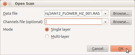
The Data file box is mandatory and must contain the filename of the scan data you wish to open. The Channels file box is optional and is only used when the specified data file is in RAS format (in this case the channels file simply names the channels that are contained in the file).

You can click on the Browse buttons to the right of the entry boxes to browse your hard drive for data and channels files, or used the drop-down to select previously opened data or channels files.

Finally, the Mode options determine how the file is opened:

• In Single layer mode, only one channel of the data file will be visible at a time, but multi-colored maps can be applied to the counts within the data.
• In Multi-layer mode, up to three channels of the data file may be visible at a time. In this mode, multi-colored maps are not available as up to three channels are assigned to the red, green and blue channels of the resulting image.

Single Layer Mode

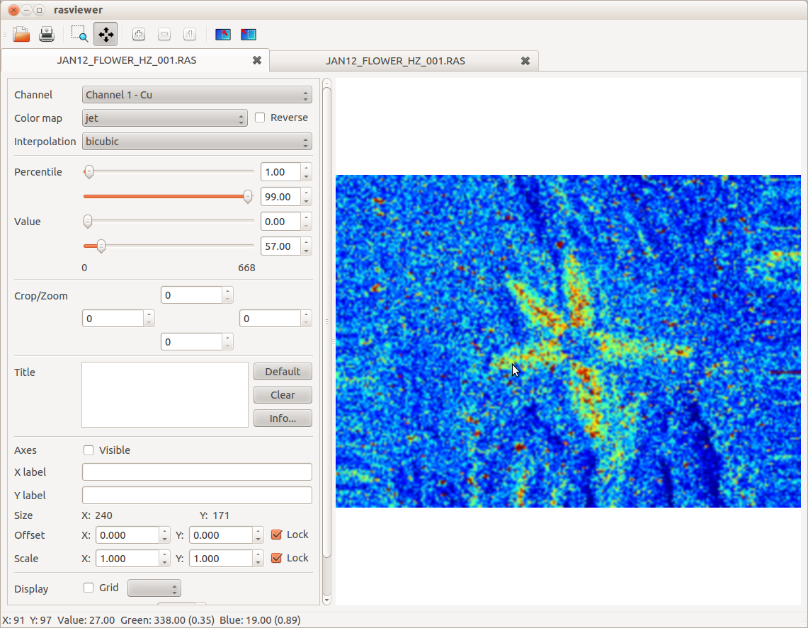
After opening a file, you should see a new tab appear in the main window. Within the tab there will be a series of controls for image manipulation and the image itself, split vertically. The first control you will most likely want to alter will be the Channel selection at the top of the controls on the left:

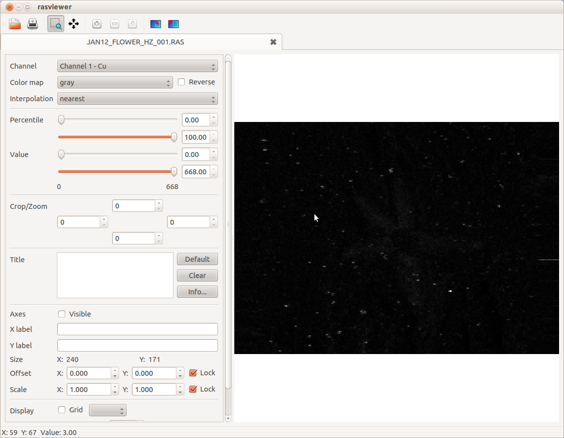
Once you have the correct channel selected, you can begin applying image manipulations such as a color map, interpolation, and percentile limits. See the following sections for more information on these controls.

Multi-Layer Mode

After opening a file in multi-layer mode, you should see a new tab appear in the main window in a very similar fashion to single layer mode. The major difference is that within the new tab are three sub-tabs labelled Red, Green, and Blue which contain controls for channel selection and percentile limits for the corresponding color channels in the output image.

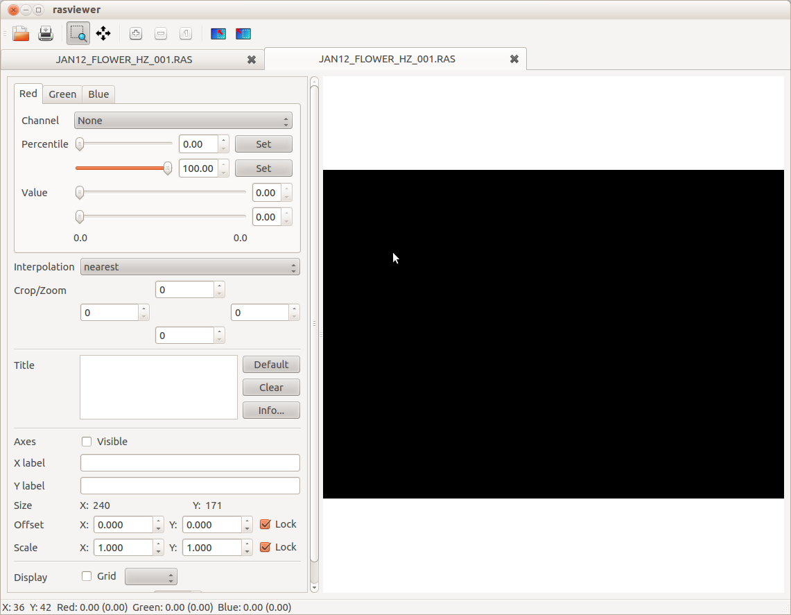
Note

Controls for color map are missing because they make little sense in multi-layer mode (the only useful color maps in this mode would be monochromatic and even then the only manipulation they could perform would be to apply a skew to the mapping from count to color).

Switching between the three color-tabs, select the channels you wish to mix into the final image, then set percentile limits. Note that in multi-layer mode, Set buttons appear next to the percentile controls which allow you to set a common percentile limit across all three color channels.

Percentile Limits

Typically, a good starting point for percentile limiting is to set the lower bound to 1% and the upper to 99%. This should bring out a reasonable degree of contrast in your image by discarding the major outliers (scanner peaks and drop-outs). You can set limits roughly by dragging the sliders, or precisely by typing values into the spin-boxes to the right of the sliders.

In multi-layer mode, a Set button appears to the right of each percentile control. When clicked, this sets the current percentile value across all color channels.

As the percentile controls are adjusted, the Value controls beneath them update to show the actual count that the selected percentile represents. You can alter the value controls instead of the percentile controls, but this is generally less useful for discarding outliers.

Note

When switching between channels, or adjusting the crop of the current channel the percentile value is maintained in preference to the actual value. In other words, if cropping the data results in a different range of values over which the percentile is calculated, then the percentile value will be maintained and the actual limits will be adjusted.

To view the count of individual points on the image, simply hover your mouse cursor over the point and view the count on the status bar at the bottom of the main window.

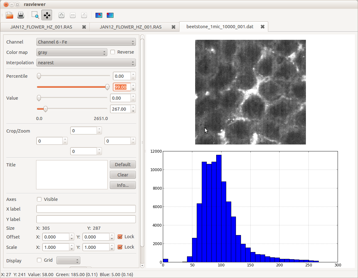
If you wish to see a histogram of the counts in the currently visible portion of the image, check the Histogram checkbox in the Display portion of the controls. The histogram is often useful in determining whether or not there are outliers (scanner peaks or dropouts) that need eliminating. For example, in the following image, the upper percentile limit has been set to 99%, eliminating the scanner peaks. However, the histogram shows an uncharacteristic peak at 0; these are scanner dropouts:

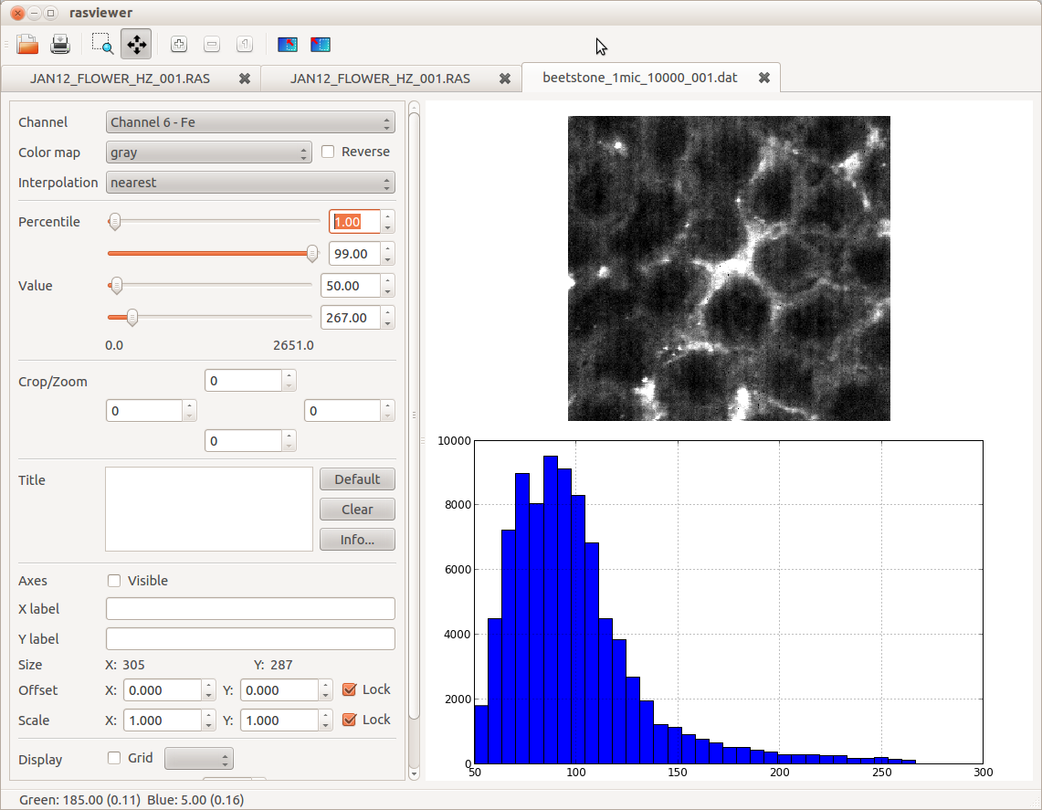
Setting the lower percentile limit to 1% will eliminate this peak and bring out the full contrast of the data. The resulting histogram also shows a nice curve with no outlying points:

Exporting Images

XXX To be written